Methodology
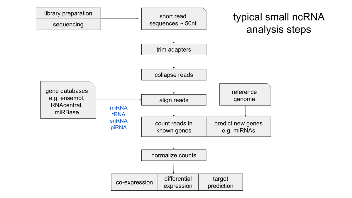
smallrnaseq is a Python package that implements some of the standard approaches for quantification and analysis of sncRNAs. This is usually implemented as part of a ‘pipeline’ that goes from raw fastq files to final counts of specific genes (e.g. coding transcripts or RNA species).
For command line usage see the ‘using smallrnaseq’ section.
Python programmers may find the various modules useful in creating their own more flexible workflows. A functional approach is used with a flat hierarchy of modules with limited use of classes.
Counting known miRNAs
This program uses the known miRNA sequences from miRBase for counting of species specific sequences. The current release used is version 22 (March 2018).
Counting isomiRs
Much miRNA expression profiling uses the read counts of all isoforms (isomiRs) of the canonical mature sequence summed together. While this may be appropriate for many cases it is also useful to consider the isoforms separately. This is true for several reasons:
- you only wish to count the exact canonical sequence.
- if the canonical mature sequence in miRBase is not even common in the tissue or samples you are studying and you wish to know this information.
- your samples contain two isoforms that differ such that one will not be detected in (for example) a PCR assay, giving an inconsistent result.
- one or more isoforms can better distinguish between sets of samples (i.e. control and disease) than the entire sum of counts.
Classifying isomiRs
Sequence variants include 5’ and 3’ trimming and extension, non-templated additions (enzymatically addition of a nucleotide to the 3’ end, i.e. adenylation, uridylation). A single read can have more than one modification so sRNAbench provided a useful non-redundant hierarchical method of classifying isomiRs. See reference below. A similar scheme has been used by Loher et al. The sRNAbench scheme is illustrated below:
isomiR counting
We have implemented the sRNAbench naming scheme. isomiR data is output
by default when the map_mirbase method is called.
If required, you can explicitly call the routine to count isomirs, assuming you have already aligned to the mirbase sequences and have a sam file. You should also provide the original read counts loaded from the csv file which is always created when the reads are collapsed.
smrna.count_isomirs(samfile, truecounts, species='bta')
References
- Barturen, G., Rueda, A., … Hackenberg, M. (2014). sRNAbench: profiling of small RNAs and its sequence variants in single or multi-species high-throughput experiments. Methods in Next Generation Sequencing, 1(1), 21–31.
- Telonis, A.G. et al., 2015. Beyond the one-locus-one-miRNA paradigm: microRNA isoforms enable deeper insights into breast cancer heterogeneity. Nucleic Acids Research, 43(19), pp.9158–9175.
- Loher,P., Londin,E.R. and Rigoutsos,I. (2014) IsomiR Expression Profiles in Human Lymphoblastoid Cell Lines Exhibit Population and Gender Dependencies. Oncotarget, 5, 8790–8802.
Counting genomic features
Counting features means counting the overlap of your reads with the locations of gene annotations (the features) in a reference genome. A short read aligner is the first step. Note that if you are aligning to a human-sized reference genome, creating the index from the fasta file can take some time. Also this process can use a lot of memory. See the section on Aligners for more information.
After read alignment to a reference genome the next step in transcriptomics is usually to count the features that each read intersects. This done using the sam or bam file generated by the aligner (e.g. bowtie) along with a gtf or gff file that stores the annotated genes - the features. These files are available for many spedcies from Ensembl. These will include annotations for non coding RNAs.
Counting features
import smallrnaseq as smrna
import pandas as pd
readcounts = pd.read_csv('counts.csv')
fcounts = smrna.count_features(samfile, gtffile, truecounts=readcounts)
This returns a pandas dataframe of the form:
                   name   reads
259         _no_feature  290705
50            _unmapped  145281
645  ENSBTAT00000060484   15162
287  ENSBTAT00000042309    6284
538  ENSBTAT00000051764    5575
...
This will merge the gtf file fields with the read counts, which can also be done explicitly using:
res = base.merge_features(fcounts, gtffile)
Novel miRNA prediction
Novel miRNAs in a species are generally those for which the mature sequence is not present in miRBase. This may be because the species has not been well studied or insufficient evidence is available to consider a sequence a real miRNA. There are problems with false positives in general for miRNA discovery from deep sequencing and this should be kept in mind when running an analysis of your reads. It is advised to use at least two algorithms for such an analysis. Most of the higher abundance miRNAs have been identified in the commonly studied species. Detection/prediction of new mirs will therefore involve looking at the low abundance (or tissue specific) forms which will need further evidence such as conservation, experimental verification and perhaps identification of function.
There are by now multiple algorithms available for predicting novel miRNAs from small RNA sequencing data. The most popular is probably miRDeep2. This algorithm is accessible via the mirdeep2 module assuming you have installed mirdeep2 as well. However we include a native algorithm in smallrnaseq for novel prediction, this is described below.
Method
The built-in method for novel prediction should be considered a somewhat ‘quick and dirty’ method at present but is relatively fast and convenient to use. The basic idea is to take clusters of reads that could be mature sequence and find suitable precursors. Structural features of each precursor are then scored using a classifier. The best candidate is selected is there is at least one. We have followed a similar approach to the miRanalyzer method.
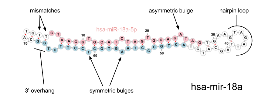
The following features are currently used in our algorithm, most are the same as those used in sRNAbench (miRanalyzer). The diagram below may help to clarify some of the terminology used.
| Feature | Description |
|---|---|
| Length | The length of the longest hairpin structure |
| Stem length | The length of the longest hairpin structure stem |
| Mfe | The mean free energy of the hairpin |
| Loop length | The number of bases in the loop of the hairpin |
| Loop GC | The GC-content of the loop |
| GC | The GC-content of the small hairpin |
| Asymmetric bulges | The number of asymmetric bulges and mismatches in the stem |
| Symmetric bulges | The number of symmetric bulges and mismatches in the stem |
| Bulges | The number of bulges in the stem |
| Longest bulge | The number of non-pairing nucleotides of the longest bulge |
| Hairpin mismatches | The number of single mismatches in the hairpin |
| Mature mismatches | The number of single mismatches in the mature microRNA region of the hairpin |
| Triplet-SVM features | All features that were proposed by Xue et al. |
Algorithm:
The basic steps for novel precursor detection are as follows.
- if multiple samples, read counts for all samples are put together using each sam file and total counts for each unique read (after collapsing the original fastq files)
- the reads are sorted by read count
- reads are clustered using cluster trees
- read clusters are themselves clustered to detect pairs within 100 nt (for animals). these are considered to be possible mature/star arms and checked for hairpin structure
- single clusters are checked for precursors by creating multiple possible precursors at the 5’ and 3’ ends and evaluating the features
- a precursor is discarded if:
- it has no hairpin
- its read cluster overlaps with the hairpin loop
- it has less than 19 bindings in the stem
- it has less than 11 bindings to the region occupied by the read cluster
- a random forest classifier/regressor trained on known positives and negatives is used to score the precursor features
- the precursor with the lowest energy and highest score is used as the most likely candidate
- for single clusters this region is considered the mature arm and the star sequence is estimated
- the list of novel miRNAs with precursor, mature, star, reads is output
Command line usage
Using the command line tool it is simply a matter of setting
novel = 1 in the config file. Reads will first be mapped to mirbase
to remove known miRNAs and also any libraries you included in the
indexes option. The novel prediction step from the command line tool
will produce a file called novel_mirna.csv in the output folder.
Code examples
from smallrnaseq import novel
import pandas as pd
#single file prediction
readcounts = pd.read_csv('countsfile.csv')
samfile = 'mysamfile.sam'
reads = utils.get_aligned_reads(samfile, readcounts)
new = novel.find_mirnas(reads, ref_fasta)
References
- Kang, W. & Friedländer, M.R., 2015. Computational Prediction of miRNA Genes from Small RNA Sequencing Data. Frontiers in Bioengineering and Biotechnology, 3, p.7.
- Hackenberg, M. et al., 2009. miRanalyzer: a microRNA detection and analysis tool for next-generation sequencing experiments. Nucleic Acids Research, 37(Web Server), pp.W68–W76.
- Friedländer, M.R. et al., 2012. miRDeep2 accurately identifies known and hundreds of novel microRNA genes in seven animal clades. Nucleic acids research, 40(1), pp.37–52.
- Shi, J. et al., 2015. mirPRo–a novel standalone program for differential expression and variation analysis of miRNAs. Scientific Reports, 5, p.14617.
- Xue, C. et al., 2005. Classification of real and pseudo microRNA precursors using local structure-sequence features and support vector machine. BMC bioinformatics, 6, p.310.
- Lopes, I.D.O.N. et al., 2014. The discriminant power of RNA features for pre-miRNA recognition. BMC bioinformatics, 15(1), p.124.